By using machine learning algorithms, we are increasingly able to use computers to perform intellectual tasks at a level approaching that of humans. Given that computers cost less than employees, many people are afraid that humans will therefore necessarily lose their jobs to computers. Contrary to this belief, in this article I show that even when a computer can perform a task more economically than a human, careful analysis suggests that humans and computers working together can sometimes yield even better business outcomes than simply replacing one with the other.

Specifically, I show how a classifier with a reject option can increase worker productivity for certain types of tasks, and I show how to construct and tune such a classifier from a simple scoring function by using two thresholds. I begin with a parable featuring the same characters as the one from Part 1 of this Machine Learning Meets Economics series. I recommend reading Part 1 first, as it sets up much of the terminology I use here.

The Case of the Augmented Humans

“What seems to be the problem?” Emily the Economist asked as she walked into Danielle the Data Scientist’s office, where she was introduced to Quinn the Quality Inspector.

“Thanks for coming, Emily,” replied Danielle. “I’m really hoping you can assist me with my latest problem. It’s similar to the one you helped me out with last time we spoke.” (Author’s note: see The Case of the Useless Model from Part 1).

“I’d be happy to give it a shot,” said Emily, “Why don’t you walk me through what you’ve done so far?”

“Sure,” replied Danielle, “Fiona the Factory Manager has a new experimental factory that produces gadgets, but the defect rate is around 25%. Quinn’s Quality Inspection group checks each gadget by hand to determine which ones should be sold and which ones should be recycled. It costs $12 to check a gadget, and the accounting system assigns her group the cost of errors: every time a gadget marked as ‘sell’ is returned by a customer (i.e. a false positive) it costs $100, and based on spot-checks, each working gadget marked as ‘recycle’ (i.e. a false negative) it costs $50. Her group works very hard to avoid the penalties so her costs are $12 per gadget.”

Quinn nodded and added, “That about captures my situation, yes. My challenge today is that Fiona wants to expand production while lowering costs, and she recommended I ask Danielle for some help with this.”

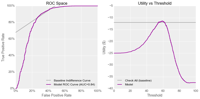
Danielle said, “I used machine learning algorithms to build a quality scanner that could tell working gadgets that should be sold (the positive class) from defective ones that should be recycled (the negative class).The best model I was able to train has an AUC of 0.84 and can achieve a lowest overall cost per gadget of $11.37. If Quinn used a quality scanner with this model instead of having her team check gadgets by hand, production could expand dramatically, and at lower cost!” Quinn frowned at this notion, so Danielle hurried along, saying “Here are the ROC and Utility curves for my model and the baseline case of checking each gadget by hand, just like we plotted last time.”

“I think I understand the problem,” said Emily. She smiled and turned to Quinn, “I assume you’re not thrilled about the idea of replacing your team with a quality scanner?”

“Indeed not,” fumed Quinn. “My team doesn’t just decide which gadgets are sold and which are recycled! We also work closely with the production group to help them improve their process based on our tests and findings. If we just used a scanner, we would essentially be using our customers to find our quality problems, which would erode our reputation in the market. Even if a scanner like Danielle’s costs less than my staff on a narrow, per-gadget basis, it would be bad for our overall process to get rid of my people.”

Danielle, a little flushed, concluded, “So that’s our problem right now, Emily. As an economist, I was hoping you could help me convince Quinn that using this model is the best thing for our business.”

“I think I can be of assistance, yes, but maybe not in the way you expect!” replied Emily. “When you analysed the model you built, you assumed that if a gadget’s score was below the threshold, it was defective and should be recycled and otherwise it should be sold, right?” Danielle nodded, so Emily continued, “Okay, but if instead of trying to replace Quinn’s team, we try to work with them, there are at least two other ways we could use this model. On top of what we’ll call your Sell/Recycle classifier, we could recycle gadgets below the threshold and have Quinn check the rest (call that the Check/Recycle classifier), or we could sell the gadgets above the threshold and have Quinn check the rest (the Sell/Check classifier). Let’s see what the utility curves look like for those situations.” Emily started tweaking equations on Danielle’s laptop.

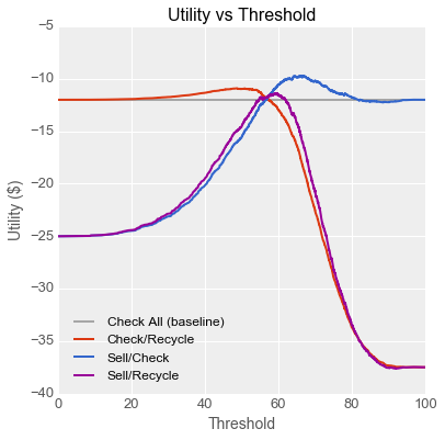
“Wow,” exclaimed Danielle, “why didn’t I think of that? If we use the model like this, Quinn’s current team can process many more gadgets than they can today, while dropping costs to under $10 per gadget!” Quinn leaned forward, very interested at this prospect.

“Just wait, I think we can do even better!” said Emily. “All three of these curves assume we just have one threshold. What if we used two thresholds, such that any gadget below the lower threshold is recycled, any gadget above the upper threshold is sold, and anything in between is checked by Quinn’s team?”

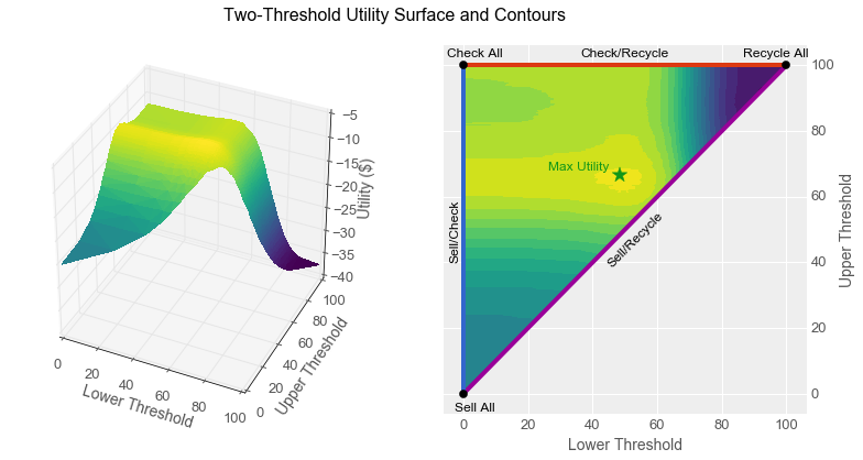
“With one threshold, we had a utility curve, but with two thresholds we have a utility surface. If we make a plot with the lower threshold on the X axis and the upper threshold on the Y axis, then the three curves we already have trace straight lines: the Sell/Recycle curve lies along the main X=Y diagonal where the lower and upper thresholds are equal. The Sell/Check curve lies along the left-hand axis where the lower threshold is 0 and the Check/Recycle curve lies along the top axis where the upper threshold is 100. Every other setting where the lower threshold is less than the upper threshold lies somewhere in the triangle. Like this.” Emily’s furious typing resulted in the following graphs. “The left-hand graph is a 3-d representation of the utility surface, and the right-hand graph is like a topographical map of that surface. Here the contours indicate utility, so they are actually indifference curves!”

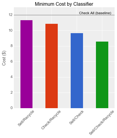
“The Sell/Check/Recycle classifier definitely beats the three other ones,” observed Emily. “You can see that the surface bulges out such that its peak isn’t along any boundary, but in the middle where the green star is. Let’s plot the utility of that point against the peak values of our other utility curves. Here we see that this combined classifier drops the cost to $8.61, for a savings of almost 30% compared to the baseline!”

Quinn jumped in at this point, asking, “This is great from a cost perspective, but what about a workload perspective?”

Danielle, already on board, fielded that question. “If we look at the distributions of scores in my testing set, which is an unbiased sample of the data, we can see how the two thresholds represented by the green star divide up the space. This graph shows that your team would only need to check one third of the gadgets, meaning you could expand production by a factor of three compared to what you do today!”

“That makes a lot of sense,” said Quinn. “If I understand correctly, by doing this we would automatically sell or recycle the gadgets about which the model is confident, the ones with very high and very low scores, and my team would manually check the ones in the middle where the model isn’t so sure. Basically the computer is catching the easy cases and the humans are working on the tough ones.”

“Exactly,” agreed Danielle, “and just like with the previous project, the model will get some wrong, but this will be outweighed by the cost savings of not having to check every single gadget.”

“I’ll get Fiona on the phone right now,” said Quinn, striding towards the door, “I want to give her the good news!”

Analysis: Classification with a Reject Option

The type of classifier described in the story above is called a classifier with a reject option in the scientific literature, because it can “reject” its input by refusing to classify it. There are other theoretical approaches to the construction of such a classifier (links are provided in the Further Reading section below), but using a simple scoring function with two thresholds is easy to analyze and implement.

The operating context of a binary classifier with a reject option consists of the utilities associated with correct and incorrect classifications for each class (@u_{tp}@, @u_{tn}@, @u_{fp}@, @u_{fn}@), the utility associated with the reject option (@u_r@), and the class distribution (@r_p@, @r_n@). Assuming the utilities associated with correct classifications are zero, we can construct a two-threshold utility surface for a scoring function with a true positive rate function @TPR(t)@ and false positive rate function @FPR(t)@:

\[utility(t_1, t_2) = u_{fn} \bigg( r_p \big(1-TPR(t_1)\big)\bigg) + u_{fp} \bigg( r_n FPR(t_2)\bigg) \\ + u_r \bigg( \big(r_n FPR(t_1)+r_p TPR(t_1) \big) - \big( r_n FPR(t_2) + r_p TPR(t_2) \big) \bigg)\]

The assumptions are actually fairly reasonable for at least some real-world business contexts. For example, for the task of online content moderation, humans use their judgement to determine whether or not user-generated content is appropriate for display on a website. The expectation of website users and operators are that inappropriate content is not displayed, so merely meeting expectations via correct classifications has a near-zero utility, whereas incorrect classifications can be shocking and have negative utility. The “reject option” for a computer performing this task would be for a human to check the content, which has a fixed utility: the cost of salaries. Given that humans are the initial source of the labels, we can model them either as perfect classifiers or assume they have a reasonably stable error rate whose costs can be added to their salaries for a fixed utility.

The utility surface defined by the equation above has some useful applications. Most obviously, and as shown in the story above, the coordinates of the global maximum for this surface indicate the threshold values which will maximize the utility of the resulting classifier.

We can also use this surface to find the optimal threshold settings under some constraints. To visualize an example of this, we can overlay a second set of contours onto the utility surface plot, which represent the utilization of the reject option as percentage of all inputs for various settings of the two thresholds. If the reject option has a capacity constraint (i.e. Quinn’s team can only check 10% of all gadgets), a contour can be traced such that every point along the curve uses the reject option at its capacity, and the maximum utility point along this curve indicates the thresholds to be used to meet the constraint.

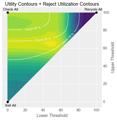
Interestingly, because every point along such a curve will use the reject option in equal measure, the threshold values for maximum utility point are independent of the cost of the reject option, so this approach can be used even when that cost is difficult to quantify. The optimal threshold values depend only on the class distribution and the ratio between the cost of false positives and false negatives, much like the slope of the indifference curve in Part 1.

Conclusions and Recommendations

Machine learning can be used to train classifiers with the potential to substantially improve the outcomes and reduce the costs associated with various types of tasks which are currently being performed by humans. In many cases, however, it will be economically optimal for computers to boost the productivity of human workers rather than to completely replace them. In this article, I have shown through a worked example at least one reasonably plausible situation where this is the case. As in many domains, when modelling the application of machine learning to the optimization of existing business processes, approaching the problem with an either/or mindset as opposed to a with/and mindset can lead to a local optimum rather than the global one.

Further Reading

As I discovered while writing this article, classification with a reject option has been studied for years and written about much more formally than I have done it here. This paper and its bibliography provide a good entry point into that literature. This paper specifically looks at the use of multiple thresholds.

⁂