Between 2011 and 2013 I wrote a popular 5-part series of articles about Datacratic's real-time bidding algorithms, and I've collected them together here for easier reading.

Part 1: is everyone pacing wrong?

I read an interesting post on the AppNexus tech blog about their campaign monitoring tools and the screenshots there almost exclusively contained various pacing measurements. Some of the graphs there looked a lot like the ones I had sketched up while trying to solve the pacing problem for our real-time bidding (RTB) client. Here are the basics of the problem: if someone gives you a fixed amount of money to run a display advertising campaign over a specific time period, it's generally advisable to spend exactly that amount of money, spread out reasonably evenly over that time-period. Over-spending could mean you're on the hook for the difference, and under-spending doesn't look great if you want repeat business. And if you don't spend it evenly, you'll get some pissed-off customers, like this guy who had his $50 budget blown in minutes. Sounds obvious, right? Apparently it's harder than it looks!

Doin' it wrong

When Datacratic first dipped its toe into RTB (real-time bidding, characterized in this sister post), the main tool at our disposal to control budget/pacing was a daily spending cap. It took about 48 hours for us to figure out that that wasn't going to work for us: depending on the types of filters we used to decide when to bid at all, we'd either not manage spend the daily budget (more on that at the bottom) or blow the budget very quickly, usually the latter. In practice this meant that we would start buying impressions at midnight (all times in this post are in Montreal local time: EST or EDT) and generally hit our cap mid-morning.

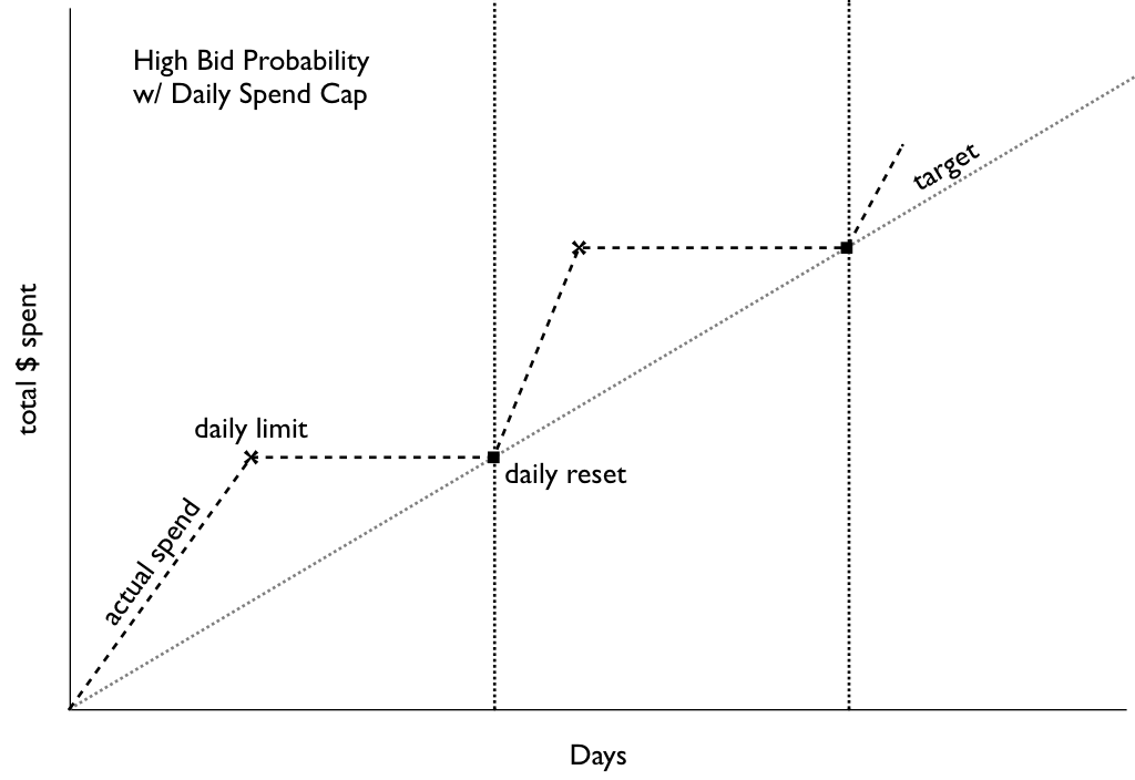
No bidding occurs after daily cap is reached

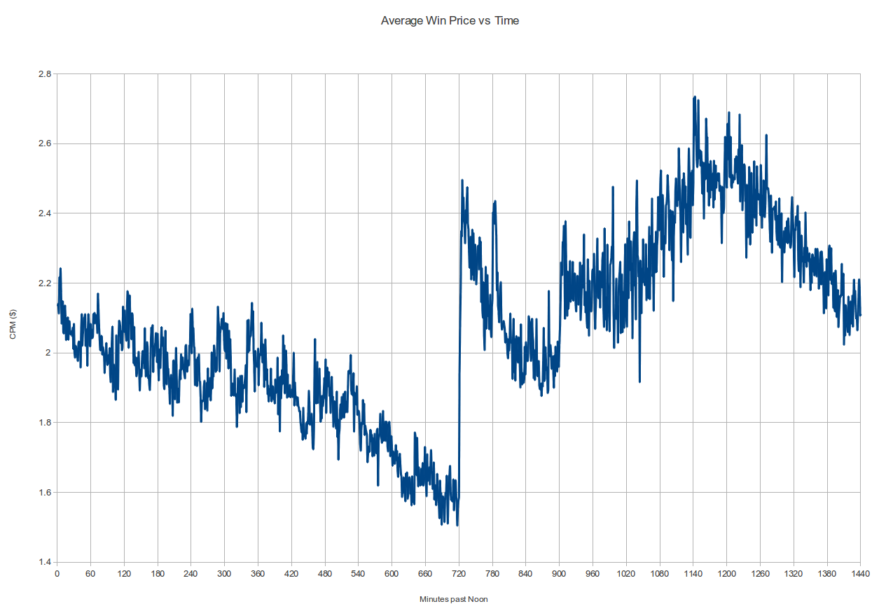
On a daily spend graph over a 30-60 day period resulting from such a policy, this would probably look just fine: you're spending the budget in the time given, and spending exactly the right amount per day. But having this sort of 'dead time' where we don't bid at all bothered us, so as soon as we spun up our own bidder we added options like "bid on X% of the request stream" and when we looked at the resulting data we noticed something really interesting: the impressions we were buying before were actually among the most expensive of the day! The average win-price graph below (i.e. what the next-highest bid was to our winning one) from a high-bidding campaign shows a pretty clear pattern: if you start at noon, the dollar cost for a thousand impressions (the CPM) generally drops until precisely midnight, then jumps something like 40%. It fluctuates a bit, hits a high in the morning and then drops down again until noon to start the cycle again. This pattern repeats day after day:

Notice the discontinuous jumps every midnight

So what's with that midnight jump? This is supposed to be an efficient marketplace, but are impressions a minute past midnight really worth 40% more than impressions 2 minutes earlier? Had we not had our initial experiences described above it might have taken us a long time to puzzle out! Our current working theory is in fact that there must be lots of bidders out there that behave just like our first one did: they have a fixed daily budget and they reset their counters at midnight. This would mean that starting at midnight, there's a whole lot more demand for impressions, and thanks to supply and demand, the price spikes way up (alternately, odds are that at least one of the many bidders coming back online is set up to bid higher than the highest-bidder in the smaller pool of 11:59PM bidders). And as bidders run out of budget throughout the day, at different times, depending on their budget and how quickly they spend it, the price drops to reduced demand. It's not obvious from the above graph but when you plot the averages over multiple days together there is a similar step at 3AM, when it's midnight on the West Coast, where a lot of other developers live and work and code:

Average Price Per Minute of the Day For the Month of August

Now there might be some other explanations for this price jump. We're in the Northeast and that impacts the composition of our bid-request stream, so maybe this is just a regional pattern (do other people see this also?) although the 3AM jump suggests otherwise. Midnight also happens to be when our bid-request volume starts its nightly dip, but that dip is gradual and isn't enough to alone explain that huge spike. Maybe some major sites have some sort of reserve price that kicks in at midnight. Or maybe everyone else is way smarter than us and noticed that click-through rates are much higher a minute past midnight than they are a minute before. I have trouble believing those explanations, though, so if anyone reading this has any thoughts on this I'd love to hear about them by email or in the comments below. Whatever the reason, it looks like if you're going to only be bidding for a few hours a day, don't choose the time-period starting at midnight and ending at 10AM!

Closed-Loop Control to the Rescue

So let's assume that this post gets a ton of coverage among the right circles and that this before/after-midnight arbitrage opportunity eventually disappears, or maybe you just want to actually spread your spending evenly throughout the day, how would you do it? As I mentioned above, we have the ability to specify a percentage of the bid-volume to bid on. The obvious way to use this capability is to see how far into the day (percentage-wise) we get with our daily budget and bid only on that percentage of the bid-request stream, thereby ensuring that we run out of budget just as midnight rolls around. In practice, though, bidding on a fixed percentage of all requests can and does result in a different amount spent each day, sometimes higher than the daily budget (if you remove the daily cap) and sometimes lower. Maybe some days you get a different volume of bid-requests, because your upstream provider is making changes. Maybe there's an outage. Maybe the composition of your bid-request stream is changing such that all of a sudden the percentage of all bid-requests that's in the geo-area you're targeting goes way up (or down). Maybe your bidding logic doesn't result in a consistent spend. All of these factors could amount to a pretty jagged spend profile:

Spend rate can change despite constant bid probability

So what's the solution? For us it's to look at this problem as a control problem and to move from open-loop control to closed-loop control. If you theorize about the appropriate bid probability, set it up and let things run for a week and look at the results later, that's basically open-loop control. If every morning you look at what the spend was the day before and adjust the coming day's bid probability accordingly, you're doing a form of closed-loop control: you're feeding back information from the output into the input. It's pretty easy to automate (at least we thought so), and once that's done, there's basically no reason not to shorten the feedback loop from daily to every few minutes. Our RTB client was designed from the ground up to facilitate this sort of thing so we were able to control spend to within 1-2% of target with the following simple control loop: every 2 minutes, set the bid probability for the subsequent 2 minutes to that which would have resulted in the 'correct spend' over the preceding 2 minutes (maybe with a bit of damping). So if for whatever reason we get 20% fewer bid requests, for example at night, the bid probability will rise so that the spend rate stays roughly constant. There are more sophisticated ways to do closed-loop control, like the PID controller which I hacked into my espresso machine, but this really basic system works pretty well:

This is actual data from around the time we activated our simple controller. Notice how Open Loop Control gives output that looks like the mountains of Mordor whereas Closed Loop Control makes it look like the fields of the Shire

Actual production data, smoothed a little bit to reveal underlying trend. Pace (blue, prob*1000) rises at night when volume drops; Spend Rate (green) stays close to target (red)

Like any good optimizer, the scheme described above does exactly what you ask it to: it tries to keep the error between 'instantaneous' spend rate and the target as close to zero as possible. If there's a full-on outage where no bidding occurs for an hour, this system will not try to make up the spend, it will just try to get the spend rate back to where it should be according to the originally-specified target, once bidding resumes:

Spend rate after outage is too low to catch up (slope remains parallel to initial target)

In order to deal with outages, as well as over- or under-spending due to accumulated error or drift from the instantaneous control system's imperfect responses, we have to dynamically adjust this spend-rate target as well. The way we've come up with to deal with this is to define the error function in terms of the original problem: continuously work to keep the spend rate at a level that will spend the remaining budget in the remaining time. This means that if there is an outage for an hour or a day, the spend rate for the rest of the campaign will be marginally higher to make up for it, without human intervention. This system also has the nice property of automatically stopping right on the dot when the remaining budget is zero:

Spend rate after outage increases to catch up (slope gets steeper as outage gets longer)

Now obviously you might not want to always have exactly the same spend rate all the time, in fact I almost guarantee that you don't. A closed-loop control system can support pretty much whatever spending profile you like. You can also use one to manipulate other variables than the bid-probability (think: the actual bid price, or the targeting criteria, or whatever other scheme your quant brain can conjure up). Finally, the astute reader will notice that the approach described above is only really useful in situations where there is more supply than your budget permits you to buy, and so you need to allocate your budget over time. The approach above won't help at all if the optimal bid probability to meet your needs is up above 100%, that is to say that even when you bid on and win everything that matches your targeting criteria, you're not able to spend your budget. That's probably a topic for a different blog post.

Follow-up: I also posted this question on Quora, where I got a few responses.

Part 2: Datacratic's RTB Algorithm

At Datacratic, we develop real-time bidding algorithms. In order to accomplish advertiser goals, our algorithms automatically take advantage of other bidders’ sub-optimal behaviour, as well as navigate around publisher price floors. These are bold claims, and we want our partners to understand how our technology works and be comfortable with it. No “trust the Black Box” value proposition for us.

First, Tell the Truth

Let’s say, for sake of illustration, that you are Datacratic's bidder. You’re configured for a 3-month direct-response campaign with a total budget of $100,000 and a target cost-per-click (CPC) of $1.00. Like every other participant in real-time auctions, you subscribe to a stream of several thousand bid requests (also known as ad calls) per second, each representing an opportunity to immediately show an ad to a particular user on a particular site. You must respond to each bid-request which matches your targeting criteria with a bid, within a few dozen milliseconds. How do you decide what amount to bid? Most real-time auctions are what are known as Vickrey, or second-price, auctions. The winner is the one who places the highest bid, but pays the amount of the second-highest bid. This type of auction was likely chosen by the designers of real-time exchange because the best strategy for bidders in such a situation is to “bid truthfully” (one of the well-known results of auction theory). This means that the bid you place should be equal to the amount that the good is worth to you. In this case the “good” is the right to show an ad. How much is that “worth”? The target CPC is $1.00, so it’s not a bad assumption that a click is worth at least that much to the advertiser. Let’s say that the average click-through rate (CTR) is 0.05% for this campaign: one out of every two thousand impressions gets clicked on. So if you win this auction, you have a 0.05% chance of getting something that is worth a dollar, and multiplying those together we can say that the expected value of winning this auction is 0.05 cents. If you’re bidding truthfully (which auction theory says you should), that’s how much you should bid. One equation you could use to come up with a bid is therefore:

bid = value = targetCPC * CTR

That’s a bit too simplistic, though, and doesn’t take advantage of the real-time nature of the exchange. We’re a predictive analytics company, so as our bidder you have access to some fancy models. These models predict, in real-time and on a bid-request by bid-request basis, the probability that this specific user will click on this specific ad in this specific context at this specific time. This means that you don’t have to use the campaign-wide average CTR when computing your bid, you can use the probability that our predictive model has generated for this request:

bid = value = targetCPC * P(click)

So far so good, but not particularly groundbreaking: where is the secret sauce, other than in the probability-of-click prediction model which is beyond the scope of this article? That predictive model is certainly part of it, but there’s actually an additional wrinkle to the above equation: it only tells you what the bid should be if you actually decide to bid. And when deciding whether or not to bid, you shouldn’t just look at the value of winning the auction, but the cost as well.

To Bid or Not To Bid, or: Cost is not Value

As I talked about in Part 1, if you just bid on every bid-request that comes your way, you’ll spend the budgeted $100,000 way ahead of the 3-month schedule. In that article I also detailed a system for spreading your spend out over time by using a closed-loop control system to vary the probability of a bid being submitted. Let’s try to take that idea further: what if instead of randomly selecting which requests to bid on, you could find a way to bid on only the best requests? I just showed a way to model the expected value of winning an auction but in this context “best” doesn’t just mean “highest value”; that’s only half the picture. As an example of this, let’s look at an importer purchasing one of two types of goods for resale. Good A has a 10% lower resale value than Good B, but it costs half as much:

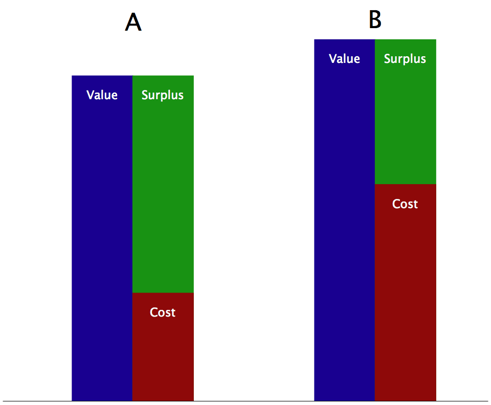
Two goods with similar values but different surpluses.

In this case the less valuable Good A is “better” because because what matters isn’t just the value or the cost but the difference between the two, or the surplus. In business this is called profit and in game theory this is usually called the payoff.

surplus = profit = payoff = value - cost

The equation above holds for the RTB context if you win the auction, but what if you don’t? In that case, you get no chance at a click, so the value is zero, and you also don’t pay anything, so the cost is zero (modulo fixed costs, which are out of the scope of this article). So for our purposes, the expected surplus is the same as above, multiplied by the probability of you actually winning the auction:

surplus = (value - cost) * P(win)

Now assuming that alongside Datacratic's click-probability predictor, you also have access to a clearing-price-predictor (again beyond the scope of the current article) that tells you for each bid-request how likely you are to win the auction at each price, you can now compute the expected surplus. (As it happens, one can also maximize this equation as a function of the bid to prove the well-known “bid truthfully” result mentioned above: the bid which gives you the highest surplus, no matter the price distribution, is equal to the value).

A surplus surface as a function of bid and value. For any given value, the maximum surplus occurs where bid=value.

So now when our closed-loop pacing control system says that in order to meet the budget requirements, you should only bid on a quarter of the request stream, you can choose to bid only on the bid-requests which have expected surpluses in the top quartile. This means that the control value is no longer the probability of bidding, but some measure of selectivity in the auctions you are willing to participate in: the lower the control value, the more selective you should be. You’re still placing the optimal bid every time, but now you’re specifically targeting the auctions where you think you will make the most profit given the target CPC, thereby increasing your chances of actually achieving a much lower CPC.

Part 3: Algorithm Meets World

In Part 2, I claimed that Datacratic’s RTB algorithm is able to take advantage of other bidders’ sub-optimal behaviour and navigate around publisher price floor in order to achieve advertiser goals. I then described the algorithm, which applies what can be called a “bid truthfully, pace economically” approach. In this second part, I show how this algorithm can in fact live up to these claims.

When you bid truthfully and pace economically, you are always trying to allocate your budget to the auctions which look like the best deals, whether that means that the user is very likely to click, or that the price is low because fewer bidders are in the running or there is no publisher price floor.

How to Take Advantage of Other Bidders’ Behaviour

In Part 1, I showed that the average win-price for RTB auctions jumps up at midnight Eastern Time and described a pacing system which, if used by everyone, would prevent this jump, by spending at a constant rate. This system works by frequently updating a control value which is interpetted as the probability of bidding on any given auction. There is an implicit assumption underlying this system though: that any two randomly-selected bids are equivalent, regardless of, for example, the time of day. So while I introduced this system by talking about variability in the clearing price over the hours of the day, the simple pacer actually ignores this fact. This did not escape all readers of my post, some of whom commented in private that if we know the price is much higher at certain times, then we just shouldn’t bid at those times! Now that I’ve described the way we compute expected surplus on a bid by bid basis, I can explain a principled way for a pacer to simultaneously handle variability in clearing prices and impression quality that doesn’t involve hardcoding hours when not to bid. All that is needed is for the pacing system to update the control value much less frequently, say once a day, and to treat the control value as a “minimum acceptable expected surplus” threshold. Consider the following graph comparing the evolution of average clearing-price and average expected surplus over a few days, noting how at midnight the price jumps and the surplus drops:

The evolution of clearing price and surplus over time.

A well-tuned, infrequently-updating pacing system will essentially draw a horizontal line across this graph, and our bidder will bid whenever the surplus is higher than this threshold. The key insight here is that the curves here represent the means of some fairly wide and skewed distributions. Even if the mean price goes up and therefore the expected surplus drops, that doesn’t mean there aren’t any “good deals” to be had: it just means there are fewer of them. By setting a hard, slowly-changing threshold, our bidder can continue bidding throughout the day, but it will probably spend less in the hour right after midnight than in the hour right before midnight. We like to say that this is taking advantage of other bidders’ sub-optimal behaviour because some bidders are irrationally piling into the market right after midnight and driving the price up. Our algorithm continues to “skim the cream”, bidding in the best-looking auctions, but does back off a bit, holding its budget in reserve for such times as other bidders have run out of money for the day. As that happens, the drop in demand causes a drop in clearing price and a concurrent rise in expected surplus, causing our bidder to spend more.

Navigating Around Publisher Price Floors

Having covered how our algorithm responds to the actions of other bidders, how about publishers? How does this system respond to publisher price floors? A price floor, or reserve price, is basically a statement by a publisher that they will not sell below a certain price. It’s almost as if a publisher is bidding on its own inventory. If there are no higher bids than the price floor, there is no transaction. If there is more than one bid above the price floor then the price floor does nothing and the winner pays the second price. If there is only one higher bid, however, that bidder wins and pays the reserve price. In this third case, the publisher gets some of the surplus from the auction that the winner would have gotten had there been no floor.

First Price	Second Price	Reserve Price	Clearing Price
5	3	(n/a)	3
5	3	2	3
5	3	4	4
5	3	6	(no transaction)

This all makes perfect sense at the micro level, as by definition if we win the auction, we were willing to pay more than we did: our bid was how much it was worth to us, and we paid the second price so the difference between the two is profit for us. Any publisher would rather that we had just paid them the entire bid amount so they could get that profit, and therefore they have an incentive to raise the price floor all the way to our bid amount to “capture back” as much of that surplus as they can. Our algorithm responds to a publisher price floor the same way it responds to the actions of other bidders causing the price to rise. At any given time, the pacer’s control value tells our bidder the minimum expected surplus required for it to bid. If a publisher raises their price floor (and if our price model captures this), the expected surplus of auctions for their impressions will drop. If it drops below the control value, we will simply not bid on those auctions at all, rather than accepting the higher price. This is what we call navigating around publisher price floors. The control value is set so that the budget will be met, and is based on the availability of surplus on the whole exchange, not just on any one publisher’s sites. In effect, this puts an upper bound on the price floor any publisher can set before losing our business, so long as we can get a higher expected surplus elsewhere. This upper bound will be lower than the value to us of winning the auction, but could still be higher than the next-highest bid, so we do give up some of the surplus to the publisher. This is pretty much the way the exchange should work: it’s a market mechanism which uses competition to divide up the surplus pie.

The control value places an upper bound on the price floor that is lower than the value.

It’s worth mentioning that at the macro level, publishers don’t necessarily sell all their inventory on a spot basis on the RTB exchange: they try to sell inventory at a much higher price on a forward contract basis ahead of time. In industry jargon, inventory sold on a forward contract basis is called “premium” and everything else is called “remnant”. Without getting too deeply into this, publishers have an incentive to put up very high floor prices so that advertisers don’t stop buying expensive premium inventory because they think they can buy the same impressions more cheaply on the spot market (i.e. as remnant inventory). The industry lingo for this effect is “cross-channel conflict”, because the remnant "channel" is perceived to be hurting the premium "channel". If a publisher is using this type of rationale to set a price floor, they will likely set it higher than the amount of our bid, rather than trying to squeeze it in between the first and second highest bids. This would translate into an expected surplus of zero, as there would be no chance of us winning the auction. Again, our algorithm just doesn’t bid on this type of auction; it certainly doesn’t raise the bid value to win an unprofitable impression. Mike on Ads has a good post about why it’s a bad idea for publishers to do this, based on some hypothetical behaviour of bidders. Our algorithm can automatically implement the types of behaviour he describes.

Part 4: Beyond Surplus

In Part 2, I described how you could compute the expected economic surplus of truthfully bidding on an impression in an RTB context. I then explained that you could use this computation to decide which bidding opportunities were “better” than others and therefore decide when to bid and and when not to bid, based on the output of a closed-loop pace control system such as the one described in Part 1.

In this post, I show that in order to maximize the economic surplus over a whole campaign, the quantity you should use on an auction-by-auction basis to decide when to bid is actually the expected return on investment (ROI) rather than the expected surplus. At Datacratic, we actually switched to an ROI-based strategy in late 2012.

Too Little of a Good Thing

The total economic surplus of a campaign can be expressed as follows:

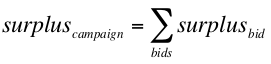
Looking at this, it makes sense that maximizing the expected surplus for each individual bid maximize the total, right? Not necessarily, because there is a constraint here: the total cost of all the bids must be equal to the budget. If by maximizing each expected per-bid surplus you end up paying more per bid, you won’t be able to bid as often, which might actually lower your total surplus. That doesn’t mean you should try to bid when the expected surplus is low, but it does mean you want to try to balance the surplus with the cost.

This problem was solved long ago by finance types, using a quantity called variously return on investment (ROI) or rate of return or yield, in order to compare the efficiency of investments against each other:

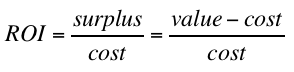
If you consider each bid to be an investment, and your closed-loop pace control system is telling you that you’re over- or under-spending, you should therefore raise or lower the minimum expected ROI threshold that you’re willing to see before bidding, rather than the minimum expected surplus threshold. In finance, this threshold is called the minimum acceptable rate of return (MARR) or hurdle rate.

A Thought Experiment

Here is a thought experiment in which an ROI-based pacing strategy outperforms a surplus-based one.

Assume a campaign with a budget of $1000 and a target cost per action (CPA) of $1 where an ‘action’ is a post-impression event like a click or conversion or video-view. Scenarios A and B both have an infinite supply of identical bid requests, differing only in their “response rate” (the percentage of the time that the impression results in the desired action) and price. Furthermore, assume that we have very accurate probability-of-action and cost predictors. Let’s say that the clearing price is less than the expected value (and thus the bid) in both scenarios, the probability of winning is 1.

	Response Rate	Value	Cost	Surplus	ROI	Spend	Imps	Actions	CPA
A	0.1%	u$1000	u$750	u$250	33%	$1000	1.333M	1333	$0.75
B	0.05%	u$500	u$250	u$250	100%	$1000	4M	2000	$0.50

The surplus is equal in both cases but scenario B, with the higher ROI, results in a lower CPA.

Now the thought experiment: how do the two strategies cope when they face an infinite alternating mix of the requests from scenarios A and B, plus some other kind of impression X with a much lower CTR and higher cost?

Pacing Strategy	A Imps	B Imps	X imps	Actions	CPA
surplus-based	1M	1M	0	1500	$0.66
ROI-based	0	4M	0	2000	$0.50

Both strategies successfully purchase no X-type impressions, as neither the surplus nor the ROI is optimal for those. The surplus-based pacing strategy, however, cannot distinguish between A-type and B-type impressions (they have the same surplus) and so buys them as they come, getting 1M of each before spending its budget. The ROI-based pacing strategy ignores the A-type impressions like the X-type, as the B-type have a higher ROI than either.

The ROI-based pacing strategy ends up with a much better CPA than the surplus-based one.

Conclusion

Advertisers, like fund managers, use ROI (or CPA as a proxy for ROI) to decide which channels or strategies they should invest in. If you are bidding truthfully and pacing by withholding your bids when some economic quantity is below some threshold, then that quantity should also be expected ROI, instead of expected surplus. This in effect treats every bid as an investment, and allocates your budget to the most efficient bids, minimizing campaign CPA and maximizing both campaign ROI and surplus.

Part 5: Shady Bidding

In Part 2, I said that in real-time bidding, we should “bid truthfully”, i.e. that you should bid whatever it is worth to you to win. To compute this truthful value, given a target cost per action (CPA) for a campaign, I said you could just multiply that target by the computed probability of seeing an action after the impression, and that would give you your bid value.

I added that by calculating an expected cost of winning an auction, you could compute the expected surplus for that auction and that to pace your spending efficiently, you would only bid truthfully when this expected surplus was above some threshold value, and not bid otherwise. This threshold value would be the output of a closed-loop pace control system whose job it is to keep the spend rate close to some target.

In Part 4, I then showed that in fact, this second claim was not optimal and that instead of setting an expected surplus threshold, you should set an expected return-on-investment (ROI) threshold.

In this final part, I show that the meaning of “bidding truthfully” can be slipperier than expected, and that you can get the same results as an ROI-based pacing strategy with a perfect expected-cost model, without even needing to use an expected-cost model.

Same Same but Different

Let’s say you’ve implemented the ROI-based strategy described in Part 4. You have an opportunity to bid on an impression which you compute has a 0.1% chance of resulting in an action such as a click or conversion. The target CPA is $1 so you’re willing to bid 1000 microdollars. Your pacing system tells you that right now, the minimum expected ROI you should accept is 50%. Do you bid or not? The answer depends on how much you think the impression will cost: if you think it will cost less than 666 micros, then yes, because any more than that and the expected ROI will be less than 50%.

Now say that you estimate that the cost of winning this auction will be 500 micros (pre-auction expected ROI of 100%) so you bid the 1000 micros and… too bad, your cost estimate was off by 50% and you paid 750 micros. Your post-auction expected ROI is now 33%, which is less than you were willing to accept before the auction. Bummer.

But wait, given that you were willing to bid 1000 micros if the cost was less than 666 micros and nothing otherwise, then you don’t actually need to estimate the cost and run the risk of being wrong: you could just bid 666 micros. The cost is determined by the next-highest bid: if it’s lower than 666 then you win and you pay less than 666 for something which was worth 1000 to you (ROI is greater than 50%, as desired!), and if it’s higher then you lose and you pay nothing (ROI not well defined). Essentially, the auction mechanism is computing the cost for you and always coming up with the right answer.

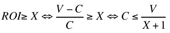
Let’s switch to symbols: under the scheme described in Part 4 (let’s call it the “truth-or-nothing” bidding policy), you’re willing to bid your expected value V when the expected ROI is X or higher and 0 otherwise. If C is the expected cost (and assuming that C < V otherwise we wouldn’t be bidding, so the P(win) is 1), then the expected ROI is (V-C)/C and the ROI is X or higher when the cost is at or lower than V/(X+1).

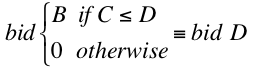
Given the mechanics of second-price auctions, if you happen to have a great cost estimator and are willing to bid some amount B when the cost C is less than or equal to D then, assuming B>D, you should be always be willing to bid D: you will win and lose the exact same auctions at exactly the same cost. We can call the policy of bidding at D when you were willing to bid at B the “shaded” bidding policy, because bid-shading is the technical term for bidding lower than you’re willing to pay. So the following bidding policies are equivalent:

Here’s a rough proof for all costs:

Cost	Truth-or-Nothing Bid	Shaded Bid	Truth-or-Nothing Win?	Shaded Win?
C > B	0	D	no	no
B>C>D	0	D	no	no
C<D	B	D	yes	yes

Putting it all together, given that X is always greater than 0 (we don’t accept a negative ROI), the following bidding policies are equivalent:

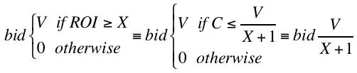
The big surprise here is that the shaded bid policy gives you the same results as the truth-or-nothing policy and you don’t actually need to compute an expected cost at all. In fact, you get the same outcomes bidding with the shaded policy as you do with the truth-or-nothing policy if you have a perfect cost model. If you have a less-than-perfect cost model, the truth-or-nothing policy could perform much worse. Given that no one has a perfect cost model and that building even a mediocre one is a lot of work, the shaded policy is clearly a pretty big improvement!

How should we reconcile this with the theory that bidding truthfully is the surplus-optimal thing to do in a single auction? The proof of this optimally boils down to the fact that for a given single auction, if you bid higher than your true value, you might overpay (i.e. get a negative surplus) and if you bid lower, you might lose out on an opportunity to get what you want at a lower cost than its value (i.e. get a positive surplus). In a context like RTB, though, where you spread out your spend over millions of auctions, it’s OK to miss an opportunity to get a bit of positive surplus, if there’s a higher-ROI opportunity coming up, so shading your bids is not a bad idea. There’s another problem with bidding truthfully, though, which comes up if you don’t actually know the true value of winning.

The Lower the Better

The problem I laid out in Part 2 of this series was one in which you had a set budget to spend over a given time period and you were trying to get actions that were worth a certain known amount. In direct-response campaigns, sometimes there is a concrete, known target CPA, but in something like a branding campaign, it can be a little fuzzier: the target CPA is not actually the value that the advertiser ascribes to getting an action, it comes out of comparisons with other channels/campaigns (on an ROI basis). In an arbitrage or variable-margin context, the "target" CPA is a maximum allowable CPA: no one will complain if the CPA is lower than the target. So in fact, you often just want the lowest CPA you can get, and the hard constraint is to spend the media budget or achieve the delivery objective. In a case like this, it’s actually very difficult to bid “truthfully”.

Conveniently, though, the result above yields a very simple approach to this type of situation. The shaded policy described above calls for bidding V/(X+1) where V is the target CPA * P(action) and X is the minimum expected ROI you’re willing to accept, according to a closed-loop pace controller, as described in Part 1. The pace controller doesn’t really know or care about ROI, though, it just outputs a control value that correlates well with spend rate, so that it can keep the pace on track. That means that we can rearrange the equations a little bit to say that for every auction:

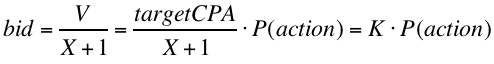
and take the output of the pace controller to be K instead of X.

Bidding in this way spends the budget while minimizes the CPA, given the constraints of liquidity and the availability of a good P(action) predictor. Given its lack of reference to ROI, value or cost, it even works when the “budget” is not dollars to be spent but impressions or actions to be bought (i.e. an arbitrage situation rather than a branding campaign). The only consideration if there is a known target CPA is to ensure that the system is able to push the CPA below the target; if it isn’t, then there is not enough liquidity to make the campaign work under the given constraints.

Conclusion

This concludes a series in which I’ve described the evolution of Datacratic’s real-time bidding algorithm over time. We started with a closed-loop control system, which has been a constant feature of our system over the years, and we’ve used it to modulate our bidding behaviour according to an ever-more sophisticated economic understanding of how to succeed in an RTB environment. The latest iteration of our algorithm is deceptively simple but by this point, theoretically quite well-grounded. Throughout this series, I haven’t put a lot of emphasis on how we actually compute the probability that an impressions being bought will result in some user action like a click or conversion but clearly, this is where the biggest value-add of our system lies. You can find out about the internals of that part of our system by watching this talk I gave at a conference in Barcelona.

⁂